“What I cannot create, I do not understand” – Richard Feynman
Following the last post about linear programming IRL, this is a summary of Ziebart et al’s 2008 paper: Maximum Entropy Inverse Reinforcement Learning . I found this is a good way for me to distill the essence of the paper. Since the Maxent algorithm is mostly cited by the later papers in IRL/imitation learning, I would like to look into details of this algorithm. Code is available at github. Hope this post can also help others who are interested in IRL.
Motivations
The paper points out the limitations of the previous algorithms including LPIRL (Ng & Russell 2000), structured maximum margin prediction (MMP, Ratliff, Bagnell & Zinkevich 2006, Apprenticeship Learning vis IRL (Abbeel & Ng 2004) about feature counts and IRL
- Both IRL and the matching of feature counts are ambiguous.
- Each policy can be optimal for many reward functions.
- many policies lead to the same feature counts.
- The ambiguity of suboptimality is unresolved.
Notations
An MDP is a tuple
- is a finite set of states.
- is a set of actions.
- is the state transition probability of landing at state : upon taking the action at state .
- is the discount factor.
- is the reward function.
Maxent
- is a trajectory.
- is the feature vector of the state .
- reward function parameters.
- probability of the trajectory to occur
- the probatility of visiting state (state visitation frequency), .
Assumptions
- The reward of a trajectory is expressed as a linearly combination with feature counts
- Principle of maximum entropy (Jaynes 1957): probability of a trajectory demonstrated by the expert is exponentially higher for higher rewards than lower rewards,
Algorithm
The Maxent algorithm learns from demonstrated expert trajectories with the objective being maximizing the likelihood of the demonstrated trajectories,
Where is the number of trajectories, is the normalization term,
Then,
And the objective is convex! (with the second term being log-sum-exp). We go ahead to differentiate the objective to find the gradients:
Since the trajectories are consist of states,
Where is the feature vector for the state . And
is the state visitation frequency for state .
So far the main body of the algorithm is described. The only thing left is to compute the state visitation frequency (SVF) vector. To do so, we can use the following dynamic programming algorithm (for convienience we use to denote SVF on state ).
We use to denote the prob of visiting at (obviously, )
- solve the MDP using value iteration with the intermediate recovered rewards to get current optimal policy .
- compute using sampled trajectories
- using DP to solve for the rest given optimal policy and the transition dynamics
For ,
- And finally.
One key things to note is that, the algorithm solves MDP in each iteration of training.
If the transition dynamics is unknown, we can actually using Monte Carlo to estimate the SVF with the trajectories. This is much more easier, so the details are omitted. Plugging the SVF back to the gradients, we can use iterative gradient descent to solve for the parameters .
Summary
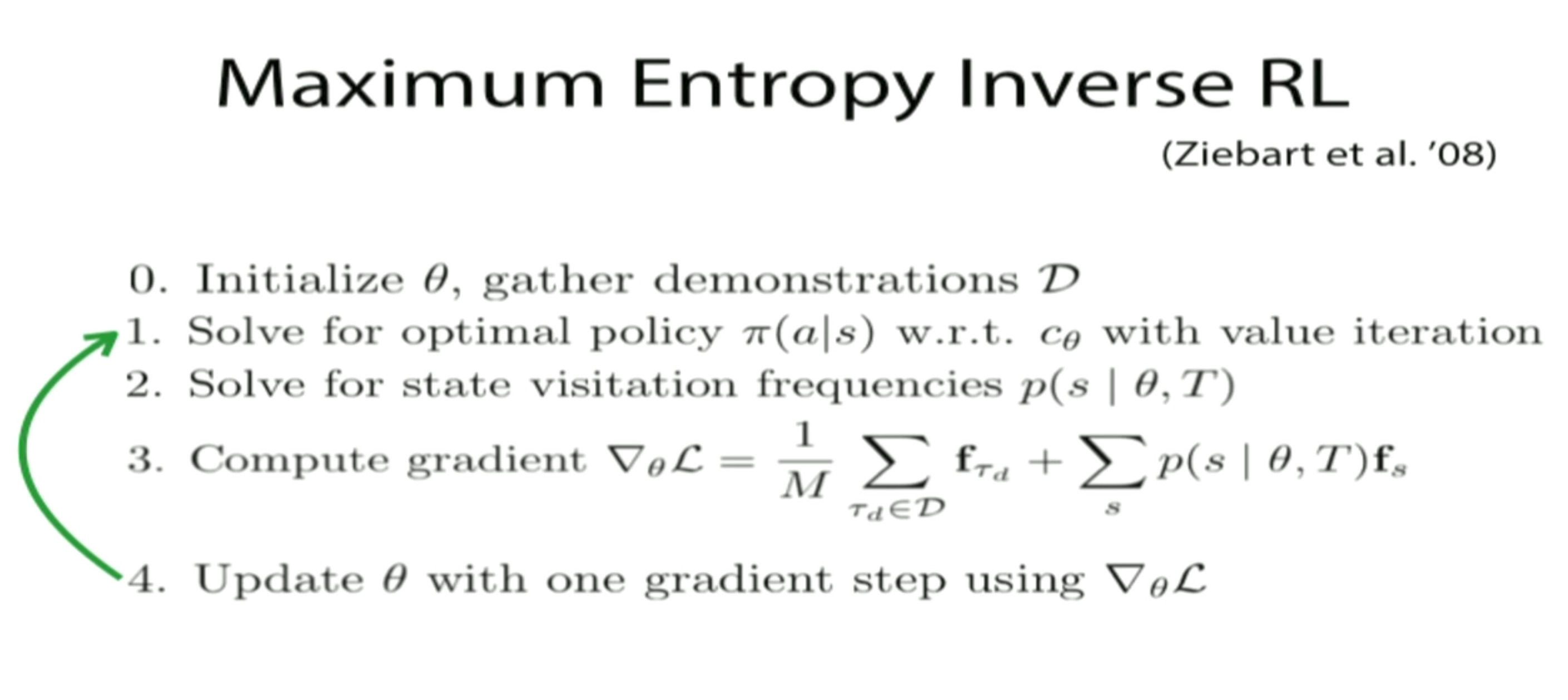
As a final summary of the algorithm, here is the slide from UC Berkeley’s CS 294, Deep Reinforcement Learning course,
Implementation & Experiments
usage: maxent_gridworld.py [-h] [-hei HEIGHT] [-wid WIDTH] [-g GAMMA]
                           [-a ACT_RANDOM] [-t N_TRAJS] [-l L_TRAJ]
                           [--rand_start] [--no-rand_start]
                           [-lr LEARNING_RATE] [-ni N_ITERS]

optional arguments:
  -h, --help            show this help message and exit
  -hei HEIGHT, --height HEIGHT
                        height of the gridworld
  -wid WIDTH, --width WIDTH
                        width of the gridworld
  -g GAMMA, --gamma GAMMA
                        discount factor
  -a ACT_RANDOM, --act_random ACT_RANDOM
                        probability of acting randomly
  -t N_TRAJS, --n_trajs N_TRAJS
                        number of expert trajectories
  -l L_TRAJ, --l_traj L_TRAJ
                        length of expert trajectory
  --rand_start          when sampling trajectories, randomly pick start
                        positions
  --no-rand_start       when sampling trajectories, fix start positions
  -lr LEARNING_RATE, --learning_rate LEARNING_RATE
                        learning rate
  -ni N_ITERS, --n_iters N_ITERS
                        number of iterations
$ python maxent_gridworld.py --height=10 --width=10 --gamma=0.8 --n_trajs=100 --l_traj=50 --no-rand_start --learning_rate=0.01 --n_iters=20
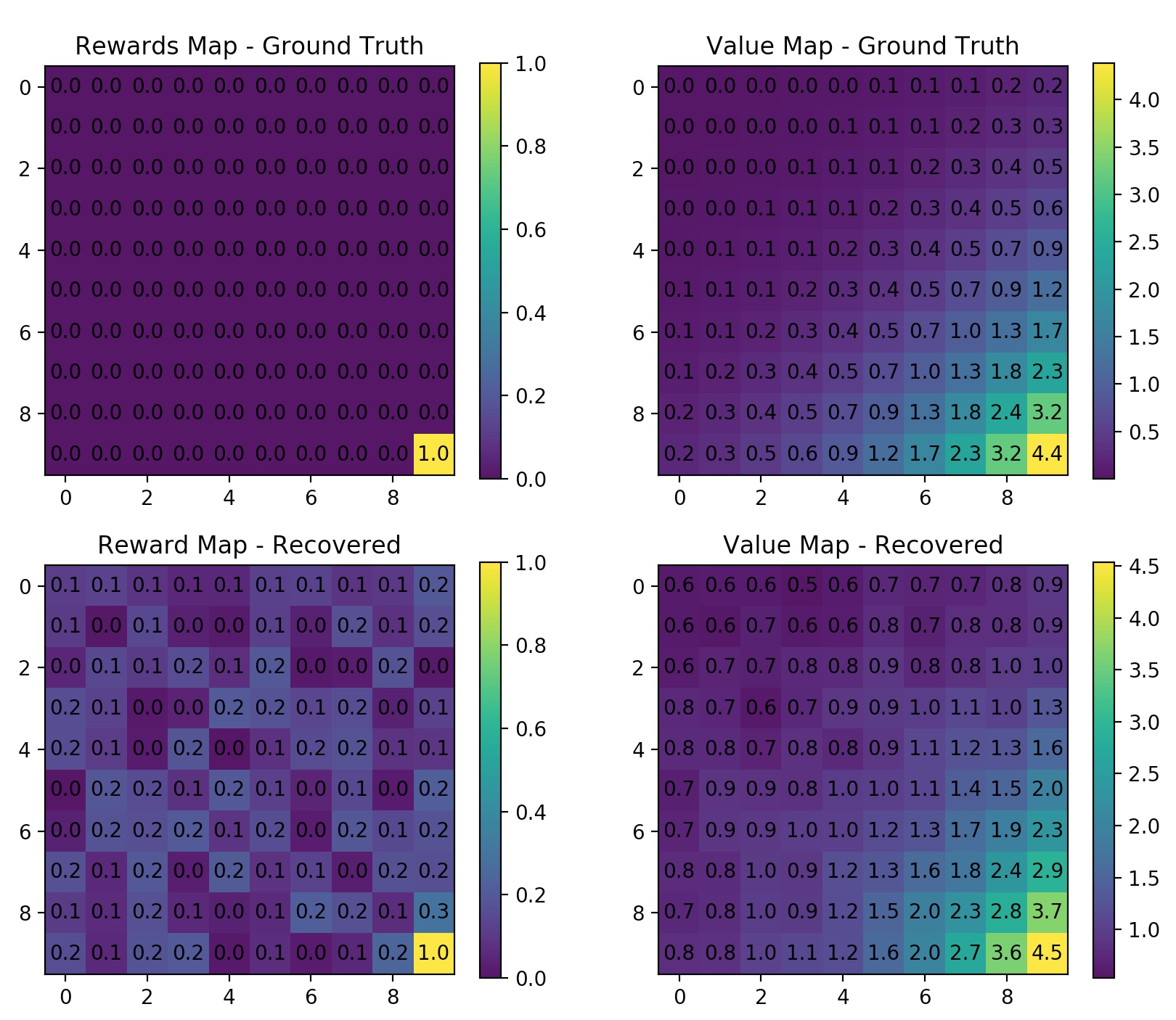
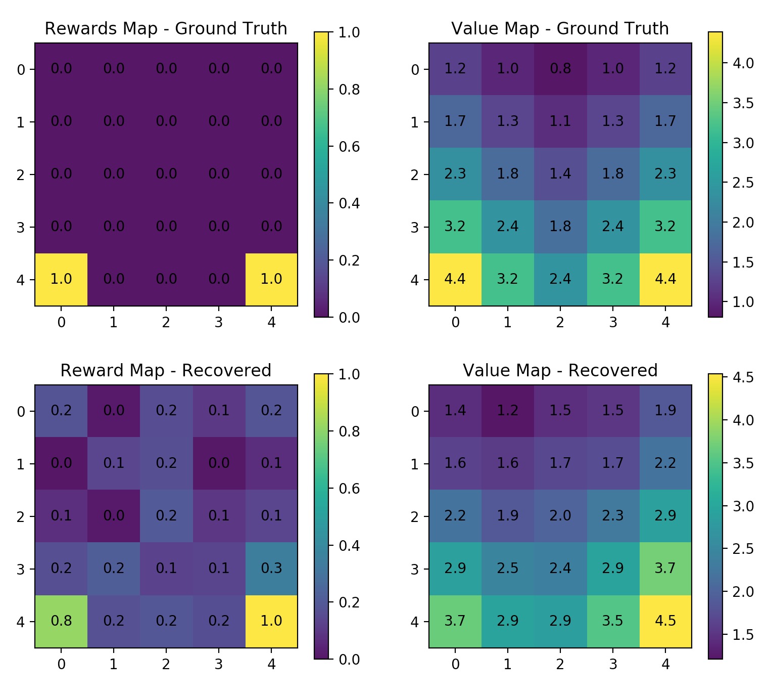
Try use 2 rewards on the gridworld. Note here I enabled random start for generating trajectories. Because if the trajectory always starts at (0,0) then they tend to go to the nearest reward and stay there.
$ python maxent_gridworld.py --gamma=0.8 --n_trajs=400 --l_traj=50 --rand_start --learning_rate=0.01 --n_iters=20
Strengths and Limitations
- Strengths
- scales to neural network costs (overcome the drawbacks of linear costs)
- efficient enough for real robots
- Limitations
- requires repeatedly solving the MDP
- assumes known dynamics
References
- Ziebart et al’s 2008 paper: Maximum Entropy Inverse Reinforcement Learning
- UCB’s CS 294 DRL course, lecture on IRL